| Cataclysmic
Variable |
| The
following description includes additional technical
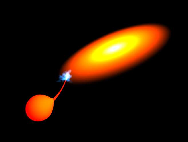
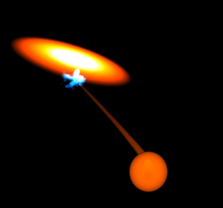
comments in brackets, the non-physicists amongst you can skip the comments in brackets. The majority of stars are not solitary like the Sun but occur in close groups in which the stars orbit about one another, bound together by gravity. Most of these stars occur in pairs as binary stars. Binary stars may exhibit all sorts of phenomena that are unknown in single star systems. One of the most dramatic is stellar accretion, in which the recipient stars either pulls material from its neighbouring star and adds it to its own mass, or the donor star throws out some of its material which is then passively scooped up by the companion. The picture above shows a type of accreting binary system, known as a cataclysmic variable (CV). In a cataclysmic variable, the two stars probably start out quite far apart, orbiting one another once every few months or years, but one of the stars eventually exhausts its own nuclear fuel. Having run out of nuclear fuel, the core of the star condenses into a very hot and very dense remnant, only about the size of the Earth, called a white dwarf. As the star stops burning fuel and 'dies' leaving the white dwarf remnant, much of its material is thrown out into space, forming a planetary nebula (so-called because in a telescope one sees a ring of gas around the white dwarf, rather like a ring of planetary material). The material that is thrown out into space forms a common envelope around both stars and imposes frictional drag on the system, causing it to lose orbital energy and so the stars move closer together, forming a close binary. The surrounding nebula is eventually ejected from the system (though some of it may fall onto the companion star, increasing its mass). In a close binary system, the stars really start to feel the tug of gravity from their companion star (remember that stars are very massive and so have strong gravitational fields). This is especially true when one of the stars is a white dwarf, since white dwarfs are so dense with a lot of mass concentrated in a small volume, that they generate a very strong gravitational field. Also if the donor star is old, perhaps a red giant, it has swollen to ten times its previous size and the outer layers of material are only loosely bound to it. (The donor star is filling its Roche lobe - the maximum extent it can have before material at its surface is more strongly attracted to the white dwarf than it is to the donor star). This arrangement favours mass transfer - the white dwarf pulls a stream of material away from its companion star onto itself. The white dwarf is essentially a parasitic star, feeding off its companion. However, if the secondary star (the one supplying matter) is larger than the primary star (the one receiving matter, i.e. the white dwarf) then the mass transfer is very rapid and catastrophic. For more steady accretion the secondary must be less massive than the white dwarf. Since the maximum size for a white dwarf is the Chandresakhar limit (thought to be around 1.4 solar masses) and most white dwarfs are less than one solar mass, most of the secondaries are red dwarfs. In the case of a cataclysmic variable, the material does not fall directly onto the white dwarf (it has too much angular momentum, that is it is rotating too fast) but instead orbits the white dwarf and spreads out into a thin disc of material that slowly falls inwards (as it slowly loses angular momentum) onto the white dwarf. Such a disc is called an accretion disc as the white dwarf accretes material from it. The material in the disc is a fluid plasma. The accretion disc is actually a huge engine for converting gravitational potential energy into radiation, and for transporting angular momentum (the bulk of the material spirals onto the white dwarf, losing angular momentum, but some of the material spirals outwards as it gains angular momentum - effectively transporting angular momentum away from the material that becomes accreted). Essentially what is happening is that as material spirals into the white dwarf, it is losing gravitational energy, just as a falling apple does, and this energy is converted into heat, so the disc becomes very hot and so glows brightly (it is a disc of plasma). A typical accretion disc of this type is about the same diameter as the Sun and the rotating material orbits the central white dwarf at speeds of about 1000 km per second, but moves inwards at only about 300 metres per second. The total mass of the disc is only about one ten thousand millionth of a solar mass (10 x E-10 SM). Notice that where the stream of material from the donor star impacts on the disc, there is a hot spot or bright spot - a local region which is hotter and brighter than the rest of the disc. Why cataclysmic variable? Though the disc shown in the picture above is in a so-called steady state, accretion discs are also prone to transient instabilities during which there is a dramatic outburst of radiation as the rate of accretion suddenly speeds up for a while, possibly increasing the brightness of the disc 100-fold in one day. Thus the brightness of the star is seen to vary. How does a Cataclysmic Variable (CV) develop? If, in a binary system, the two stars are close together in their orbits, then as the older companion expands to a red giant stage (or even a supergiant stage), it may push its tenuous outer envelope far from its own centre of gravity and closer to the centre of gravity of its younger companion. The red giant is said to overflow its Roche lobe. (The Roche lobe is the boundary which is the furthest distance material can be from one star before being more strongly attracted to the other star in a binary system). When this happens, the material, which is now loosely bound to the red giant, will be attracted toward the younger companion star, which pulls the material from the red giant with its gravitational field. Material starts to stream from the bloated red giant onto the smaller companion - a process known as mass transfer. As material streams from the red giant onto its smaller companion, conservation of angular momentum causes the stars to spiral in toward one another and the distance between them decreases. This makes matters worse, because as the distance between the two stars decreases, the red giant's Roche lobe decreases in radius and the red giant overflows its Roche lobe more and more, dumping more and more material onto its companion star. Within a few years, the red giant will have dumped almost its entire envelope onto its companion, but the companion star cannot possibly add this much material to its own atmosphere this quickly and the excess material forms a greatly distended envelope that encloses both stars. This gaseous envelope imposes drag on the two stars as they move in their orbits around one another. This braking effect causes the stars to move even closer together. Like a propeller the two stars spin faster and faster (like an ice-skater pulling in their arms) and spin off the excess material which expands out as a particular type of planetary nebula. When all this excess material has been spun off, the old red giant is now reduced to its stellar core remnant, which will be white dwarf. Nuclear burning will cease as the star has lost its fuel. However, the white dwarf may gain a new lease of life. Since it is compact and very dense, it has a very strong gravitational field, whilst its companion is now somewhat overweight and distended with the extra material it has acquired. Furthermore, the two stars are now very close together. Now the young companion overflows its Roche lobe and material starts to stream back toward the white dwarf. This is generally a more leisurely and controlled affair than when the red giant rapidly dumped its envelope, and the jet of material starts to orbit the white dwarf and eventually it forms an accretion disc. As material slowly spirals onto the white dwarf, the material heats up more and more as it accumulates on the surface of the white dwarf. Every 10 000 to 100 000 years or so, enough material accumulates to generate sufficient heat and pressure for nuclear fusion and the material suddenly ignites as it burns, blasting much of it into space. This causes the star system to brighten by as much as 100 000 times over a period as short as a few days. Such a star is called a nova, and is undergoing a nova outburst. These nova outbursts grant the white dwarf a new lease of life, as it feeds like a parasite upon its companion star. Eventually, however, the white dwarf may put on more weight than it can handle, as it adds the material to itself - if the mass of the white dwarf exceeds the Chandrasekhar limit (about 1.4 solar masses) then it is in big trouble! It can no longer support itself and it suddenly collapses in a tremendous supernova explosion (a type I supernova). Although the white dwarf may possibly collapse to a neutron star or black hole, the most likely outcome appears to be its total destruction as it detonates in a tremendous fireball! As the secondary loses mass and shrinks it may lose contact with its Roche lobe and mass transfer will cease, unless something acts to shrink the orbital and hence shrink the Roche lobe diameter such that the secondary once again overflows and mass transfer continues. Shrinking the orbit requires a loss of orbital angular momentum. Since angular momentum is conserved, something must carry momentum away from the system. For binaries with an orbital period (the time taken to complete one orbit) greater than about 3 hours, the main mechanism thought to act is magnetic breaking. If the red dwarf is locked into synchronous rotation (that is it spins at the same rate that it orbits) then it will be spinning very fast (hours rather than the days it would take for a solitary red dwarf to spin or rotate on its axis) and so will generate a very strong magnetic field. Charged particles will spiral along the magnetic field lines which are also dragged around the star, propelling the particles away from the star in a sling-shot mechanism. These particles take much angular momentum with them. So, how does the red dwarf become locked into a synchronous orbit in the first place? The gravitational attraction between two spinning stars in a close orbit causes tidal friction within the atmospheres of stars with convective atmospheres. Small stars like red dwarfs have convective atmospheres and so experience large tidal forces which drags on the star until it always shows the same face to its partner, and thus its spin period equals its orbital period and the orbit is synchronous. Binary stars in which both partners are small main sequence stars will synchronise rapidly (unless a third body perturbs their motion by its gravitational pull) long before either reaches the red giant stage (indeed perhaps before they reach the main sequence). Furthermore, if a star is initially spinning faster than it orbits, then the tide will lag behind its motion and the orbit will decay. Conversely, if the star is spinning slower than it orbits, then the tide will lead and this will cause the orbit to enlarge. this happens until the spin period equals the orbital period. For stars with convective envelopes, the orbits will also circularise (change from elliptic to circular) if the orbital period is less than about 8 days. Very massive stars, such as O class stars, are not expected to have convective envelopes and they are subject to weaker tidal forces and are also much shorter lived and pairs of such stars may never synchronise or circularise their orbits, unless their orbital periods are very short, less than about 2 days for O stars. After the disturbances of a star becoming a red giant and the formation of a planetary nebula generally leave behind a rapidly rotating stellar remnant, such as a white dwarf. White dwarfs are often also highly magnetic and interactions between the magnetic fields of the two stars (like two bar magnets interacting) may also cause locking and orbital synchronisation, in which case both stars may synchronise their orbits. However, during mass transfer the white dwarf may spin up if the transferring matter is not able to lose all of its excess angular momentum prior to accretion. The maximum orbital period of cataclysmic variables (a red dwarf secondary supplying matter to a white dwarf primary) is about 10 hours. This is because the larger the orbital separation, the larger the Roche lobe diameter and the heavier the secondary star needed to fill it, in order for mass transfer to occur by Roche lobe overflow. However, stars more massive than their white dwarf partner transfer matter catastrophically and are not observed as stable cataclysmic variables (CVs). This 10 hours period is the long-period cut-off. We also need to explain the so-called period gap between 2 and 3 hours. There are very few CVs within this orbital range. CVs with periods below 3 hours have mass transfer rates only about one-tenth of those expected when magnetic breaking shrinks the Roche lobe of the secondary. In magnetic breaking, we have a mass transfer rate of about 10^-9 to 10^-8 (one to ten billionths) of a solar mass per year, but below the period gap the mass transfer rate is only about 10^-10 (one tenth of a billion) solar masses per year. This lower mass transfer is thought to be driven by gravitational breaking due to loss of orbital energy as a result of gravitational radiation carrying away energy as ripples in space and time, i.e. as gravitational waves. (This is not to be confused with gravity waves on the surface of water!). Gravitational waves become stronger as the gravitational force strengthens, which it does the closer the stars are to one-another. This loss of orbital energy causes the stars to spiral in towards one-another: their orbital separation increases as the orbital period increases. It is worth noting that some cataclysmic variables have secondary stars which meet the criteria to be classed as brown dwarfs. These secondaries would have accreted some mass from the primary when the latter went through its red dwarf stage. The brown dwarf may have been engulfed by the expanding envelope of its red giant companion, but the propeller action of the brown dwarf and red giant core would have helped to eject this common envelope as a planetary nebula. Brown dwarfs seem able to survive this trauma and their atmospheres may contain elements from deep within the red giant. This raises several interesting possibilities if the brown dwarf is close to the red dwarf/brown dwarf boundary. It may have begun as a red dwarf but lost sufficient mass to its white dwarf partner to become a cooling brown dwarf, or it may have begun as a brown dwarf and gained enough mass from the red giant to initiate a second round of thermonuclear burning. it is also generally assumed that the inert cores of red dwarfs ensures that they have weak magnetic fields, in which case there may be no spin synchronisation with the white dwarf due to insufficient interactions between their magnetic fields. What follows is a more technical description of certain features of cataclysmic variables, for those who are interested in taking their understanding to a deeper level. Observing Cataclysmic Variables 1. Light-curves Observing accretion discs directly is difficult, and although advances in telescopes will enable more to be seen with increasing clarity, often they are too far and too dim to be seen. Additionally, depending on how the system is tilted relative to the viewer (and angle called the inclination of the binary system) not all of the disc can be seen - a 2D structure might need to be inferred from a 1D view. Observation of a large number of discs can overcome these difficulties, but each disc is also unique and each may exhibit different characteristics. One way to infer information is to study the light-curve. The binary is observed throughout several complete orbits and the variation in observed light intensity is plotted against time. Below is a Pov-Ray model of an accreting binary that we shall use as an example (the geometry is not meant to be exact, but is approximately correct): |
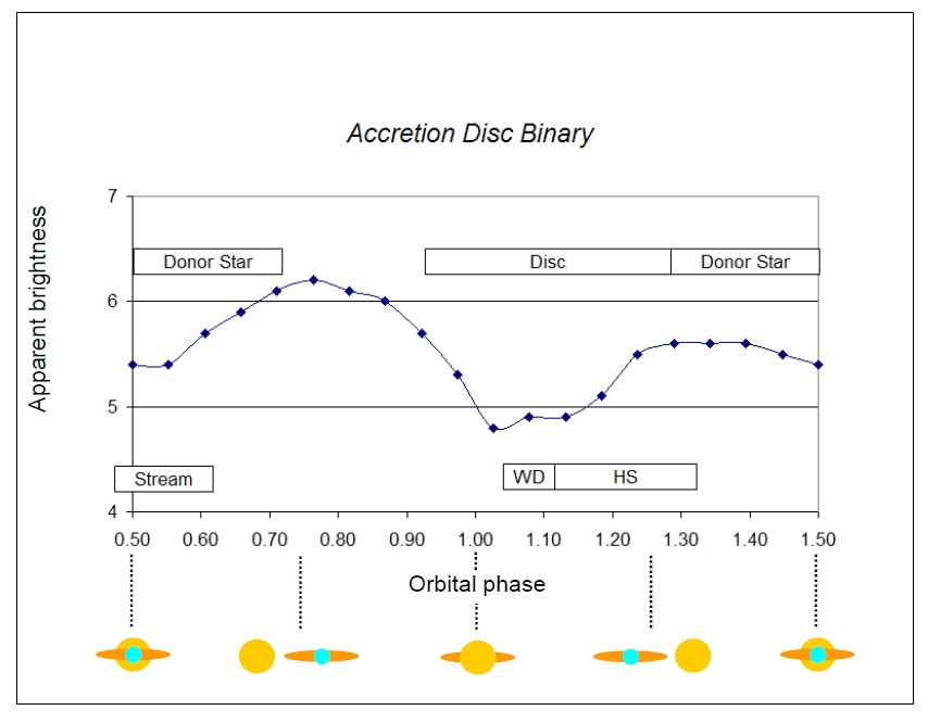
| Note
that to compare these two graphs you have to compare
identical phases. The bottom graph spans phases 0.5 to 1.5, whereas the top graph spans phases 0.9 to 1.9. To understand these graphs imagine a long line of identical graphs joined end-to-end, each link in this chain of graphs represents a single orbit. A phase from any value to that same value + 1 also spans a complete orbit! In both cases we have used the convention of setting the eclipse of the white dwarf to phase 1.0 (and hence to 0, 2, 3, 4, ... also). Thus, the point at phase 1.8 on the top graph, which is the orbital hump is equivalent to phase 0.8 on the bottom diagram. We can fix the horizontal scale wherever we like, and not everyone uses the same start and end phase for this axis! I did those just to get you used to such graphs, however, for convenience I have rescaled the axes on the graph of our model to match the actual data for Z-Cha, this rescaled graph is shown below. Looking at it you can see the similarities more clearly. So you see, it is possible to tell a lot even without a clear photographic image! There are additional techniques that may be used and we consider these next. |
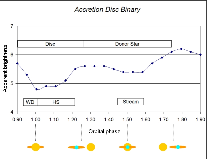
| The
inclination
of a binary is the angle it makes with the observer, and
is equal to 90 degrees if the binary 9disc) is edge-on and zero degrees if it is face-on (like looking down from above). If the disc is observed edge-on, then the donor star will eclipse the various structures - hot spot, accretion stream, white dwarf companion (in the centre of the disc) and the disc itself as it completes its orbit. The way the light-curve varies reveals the structure of the system. For illustration, we can study the average intensity of the pixels in each animation frame (as we did for the simpler case of the contact binary). The result is shown below, in which apparent brightness 9in arbitrary units) is plotted against orbital phase. The orbital phase is the number of whole or fractional orbits completed, from the point we begin recording, which conventionally is chosen as the point at which the larger star eclipses the smaller star and the light-curve is at a minimum. The phase keeps counting indefinitely, thus the smaller star gets eclipsed at phase 0, 1, 2, 3, ... etc. At these phases the larger (donor) star is pointing straight at us, and the white dwarf is eclipsed. |
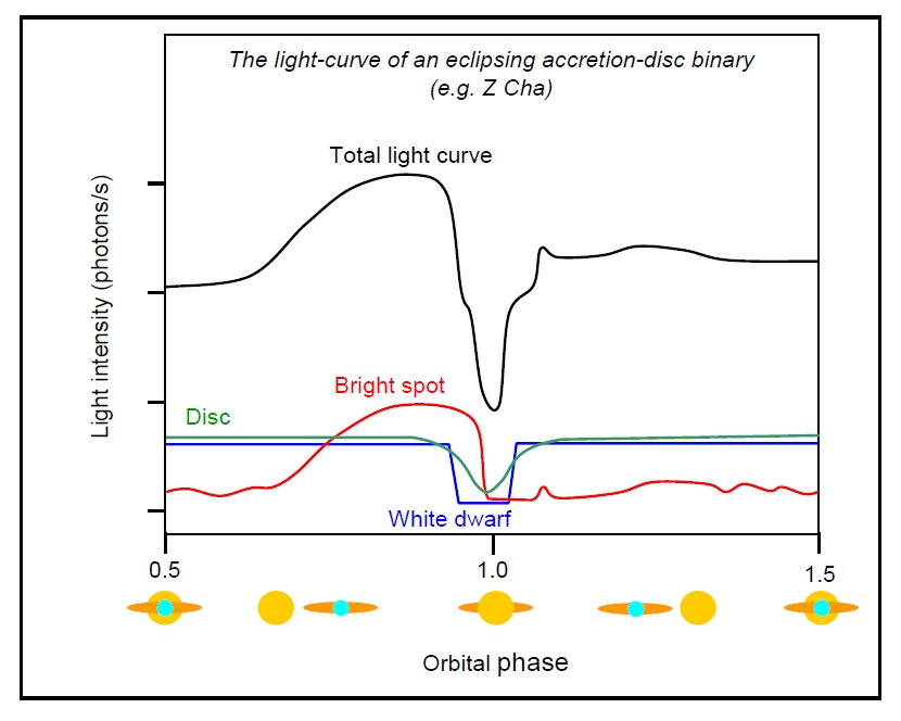
| Compare
this to the sketch of actual publsihed data obtained for
the system Z Cha. The similarities are striking. The bars in the picture above indicate the phases at which the following structures are eclipsed: WD, white dwarf; HS, hot spot; and disc by the donor star, and the donor star being partially eclipsed itself by the accretion disc (note that the disc may be more-or-less opaque depending on the system and the rate of mass transfer). The bright spot (hot spot, HS) causes the orbital hump (phase 1.8 in the above diagram, phase 0.8 in the below diagram, which are equivalent phases!) as it is on the near-side of the disc. Hot spots may account for up to 30% of the total light emitted by the system. (Note, our spot varies in shape as the stars rotate to add more realistic variation). The minimum of the light-curve occurs when either the white dwarf (WD) or hot spot (HS) is eclipsed, or both if this is observed. There is a shallower, but more prolonged dip due to the accretion disc being eclipsed (how broad this dip is will depend on the relative sizes of the donor star and the disc). In reality, we must do this modelling process in reverse - start with the light-curve and deduce the structure. In the example below, the various components making up the total light-curve have been teased apart to show the contributions from eclipsing the white dwarf, hot spot and disc. |
| Pov-Ray
model of a cataclysmic variable: above, inclination = 57
degrees; below, inclination = 90 degrees |
| Notice
that the second orbital hump is much smaller. To what
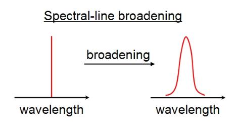
extent the bright spot can be seen when it is in the far-side of the disc depends on the thickness and opacity of the disc. The disc might be almost transparent, which may produce a double-humped curve. [The angle that the donor (secondary) makes to the white dwarf, and the degree to which it deviates from spherical, also affects the height of the second hump. However, it is assumed that the tidal bulge (see binary stars) of the donor star faces straight towards the white dwarf (primary) due to tidal locking. Is it possible that sometimes the secondary star gets dragged around or distorted by drag as it rotates? Perhaps, but we assume that the tidal bulge still faces the partner star, which draws it out, however there may be other factors distorting the shape of the secondary, apart from the Roche potential.] Discs may also be warped and of differing thickness (often being thicker on the outer rim). Not all factors affecting the specific form of the light-curve are understood. U Gem shows one orbital hump and only the bright spot is eclipsed - the white dwarf is not eclipsed, suggesting that the disc is inclined at a lower angle (Z Cha is almost edge-on, with an inclination of 82 degrees, but U Gem has an inclination of 70 degrees and so the secondary may miss the white dwarf which remains visible throughout the orbit). WZ Sge has a double-hump and perhaps has a more translucent disc or an odd-shaped secondary star. Our model had a moderately translucent disc and so the secondary hump is quite noticeable. Adjusting several model parameters readily changes the height of the second hump. 2. Eclipse Mapping What we have done so far is a rather crude attempt to obtain a lightcurve from a model that fits the actual data. The method of doing this is called eclipse mapping. Since we do not know the actual 2D or 3D representation of the disc and other system components, we can never be sure that our model is correct since several different models may give equally good fits to the data. That is several different Pov-Ray models may produce light-curves that are close to the real light-curve (such as that of Z Cha). In fact there are an infinite number of such models, as a result of losing information in going from a 2D disc to a 1D light-curve! However, we can choose the model which makes fewest assumptions, that is the simplest one, such as a circular disc which becomes cooler towards the edge equally in all (radial) directions but with a bright-spot. This model is actually the most likely, since it imposes less order on the system, and we should not impose additional order or constraints without good reason. For example why should we not assume that the disc is circular? In the most 'random' case circular is more likely than any other shape (and there are good theoretical reasons to assume a circular disc). What we are doing is minimising the order, that is maximising the entropy of the model. Each time we try a model, we can subtract the observed light-curve from the predicted light-curve and see what is left. The aim would be to get the remaining difference as close to zero as possible, and this may require that we repeatedly modify or tweak the model, in an intelligent way, to gradually improve the match in a process of iteration. Entropy is a measure of 'randomness' or 'disorder' and more specifically a measure of how many ways we can derive the model from basic processes - for example if we used an elliptical disc then we would have to decide whether the long axis points towards the donor star or is at right angles or some other angle to it - this is a complexity that decreases the entropy 9i.e. we need more information to describe the disc) when what we ought to do, in the absence of evidence to suggest an elliptical disc, is maximise the entropy and assume a circular disc. However, as we shall see later there is evidence that discs may indeed be elliptical in some circumstances. What we are doing is using a maximum entropy method (MEM). In practice there are ways to do this mathematically. In general we pick the light-curve with fewest unusual features, that is the smoothest curve. In particular, we have assumed a radial distribution of temperature within the disc, so that it gets hotter toward the centre in the same manner for all radii, that is the disc is not patchy. There is no reason to assume a significantly and irregularly patchy disc (which would not give a smooth light-curve). The simplest, or maximum entropy case, is the default image and from those models (the model images) which accurately reproduce the observed data (the real image), we chose the one most like the default image. 'Image' in this case refers to a 1D light-curve. However, the mathematical approach also applies to 2D photographic images. When we take a photograph of a distant star, for example, the photo is never a true representation. Even if our telescope is perfectly and optimally focused, the image is still 'blurred' by quantum mechanical effects (the photon is governed by a wave rather than acting as a perfect particle and so its pathway through the optics is never exactly predictable). There is a point-spread function (PSF), a mathematical equation which determines how a perfect point of light spreads or 'blurs' in the image. We can obtain this for our camera (say a CCD camera) by taking a long-exposure shot of a star, which being so far away is essentially a perfect point of light. Multiplying the 'true image' by the PSF gives the final image we observe. This is mathematical process called convolution. Given the final image and the PSF our aim would be to work backwards and try to obtain the true image in a mathematical process of deconvolution. This can never be perfect, so we can never obtain the true image with certainty, but by maximising entropy we can obtain the most likely representation (assuming photons enter different cells on our digital CCD sensor at random, that is with fewest constraints or assumptions). The end result of deconvolution is a sharper image than the camera was capable of taking! (We can validate the method by taking well-focused images and blurring them further with our own PSF and then work backwards (deconvolve) to see how close the final image is to the original). The method works just as well whether the 'image' is a 2D image or a 1D light-curve or some other signal spectrum. Thus, using MEM it is possible to find the most likely model that fits the observed light-curve, in the light of current knowledge. (For example, if other measurements suggested a warped disc, then we would be correct to factor that in to our default model). This is not ideal, but it is a useful tool. (The ideal would be detailed observations from up-close from all angles, such as by flying past in a spaceship whilst taking measurements). Furthermore, we can separate out the observed light-intensity into long wavelengths (red light) and short wavelengths (blue or ultraviolet light), Cooler objects emit more redder light. The hot spot emits white or blue light, but the cooler disc emits redder light, with the cooler edge of the disc emitting the reddest light. The centre of the disc may emit white or blue light, where it is heated up most by falling in and also from being irradiated by the white dwarf. Thus, a blue-light curve might reveal the eclipsing of the hot spot and the white dwarf, whilst a red-light curve might reveal an eclipse of the disc. We can then try to fit each component curve to a model separately. 3. Doppler Tomography and Spectral Lines Apart from light intensity varying over time, observing the light can give us much more information. Breaking down the light detected into a spectrum (a graph of colour or wavelength versus intensity) we can pick-out gaps due to spectral absorption, or bright lines due to spectral emission. Such spectral lines reveal a wealth of information. The frequencies or wavelengths at which they occur tell us what elements are present and their width can tell us such things as the temperature of the emitting material. Additionally, known spectral lines may occur at slightly redder or bluer wavelengths than in the laboratory, which is due to the Doppler effect. What is the Doppler effect? Imagine racing over water on a speed-boat. If you move toward the waves (that is if you move away from shore if the waves are incoming) and count the number of waves that pass every minute, obtaining the wave frequency, then you will get a larger number than if you turn around and speed toward shore in the same direction in which the waves are traveling. You will get a bumpier ride going away from the shore than when you return. If these were sound waves, then as you approach the waves fast, or they approach you fast, again you detect a higher frequency or a higher pitch than if the waves are moving past you more slowly. Thus, when a speeding ambulance approaches you, then its siren has a higher pitch, but when it passes you and moves away from you, the siren suddenly drops in pitch. This is the Doppler shift or Doppler effect. Similarly with light waves, if a luminous source is moving towards you, then the light waves it emits (and their spectral lines) appear to have a higher frequency, that is a shorter wavelength, and so the light appears blue-shifted. If the source is moving away from you, then it appears red-shifted. When you look at a revolving accretion disc edge-on and that disc is, say, rotating clockwise, then the right-hand edge is moving towards you and is blue-shifted, whilst the left-hand edge is moving away and is red-shifted. Furthermore, the amount of the shift depends on how fast the disc is rotating (the disc as a whole may also be moving). By looking at the shift in spectral lines we can obtain a velocity profile or velocity map of plasma within the disc. The shift in a spectral line is thus proportional to its velocity in the line-of-sight for a disc seen edge-on. The velocity of material in a disc ranges from a few hundred to several thousand km/s which produces readily detectable wavelength shifts of a few hundredths to tens of nanometres. Spectral line broadening. Line broadening is a general feature of spectral lines. If you recall how spectra are produced (see atomic spectra) by an electron transition in an atom or molecule (such that the electron jumps up by a well-defined amount of energy in absorption and drops down by a well-defined amount of energy in emission) then you will know that we expect to see a sharp spike. Quantum mechanics means that an electron in an atom or molecule can only lose or gain certain well-defined amounts of energy - the energy is quantised and changes by discrete amounts called quanta. When an electron makes such a downward jump, by losing energy, then it emits a photon carrying exactly the right amount of energy and so would produce a perfect spike in the spectrum. However, reality is not so simple. Several mechanisms broaden the spectral line from a spike into a more bell-shaped curve with a well-defined width (line broadening): |
| The
velocities of disc material can be estimated by assuming
that the material follows orbits described by Kepler's laws of orbital motion. These are Keplerian orbits. In a Keplerian orbit, such as a planet in stable orbit around the Sun, the wider the orbit (the further the planet or disc material is from the central star) the more slowly it orbits. We explained this by the fact that as matter falls into the central star, it speeds up as gravitational potential energy is converted into kinetic energy. The inner disc rotates more quickly, sliding past the outer disc (though the velocity change from one region to an adjacent region is small). However, the velocities of the outermost disc region are 10-30% lower than those predicted by Keplerian orbits, which suggests that the donor star may be perturbing the outer disc and dragging upon it. Note the high velocities of material in the disc, these velocities are supersonic. S-Waves - If we take the spectrum, that is a graph of wavelength (horizontal axis) against light intensity (vertical axis) at regular time-intervals over one complete orbit and then stack these plots on top of one-another (down the page) then we see something interesting: the double-peak snakes across in a sinusoidal fashion, shifting back and forth in wavelength during a complete orbit. This is because, although the double peak results from rotation of the disc about the central white dwarf, the white dwarf and its accompanying disc rotate as a whole about the centre of mass of the binary system, causing the wavelengths of the double-peak to Doppler shift during the course of an orbit. Considering the bright spot, this also forms a sinusoidal curve or s-wave in this manner, except it is single-peaked, since the bright spot is either coming towards us or away from us, not both together as it only occurs on one side of the disc. Other features also produce s-waves, such as lines from the white dwarf and donor star, though these are generally fainter - the disc and bright-spot dominate the emission. The result is illustrated below: |
| Several
physical mechanisms broaden spectral lines, such as: Natural broadening - quantum mechanics tells us that the longer a state exists for, the greater the uncertainty in its energy (as normally measured by strong measurements). When an electron in an atom gains energy the atom is said to be in an excited state. Typically this state lasts only about 10 billionths of a second before the electron loses the energy again, say by emitting a photon which contributes to a spectral line. The fact that this excited state is so ephemeral means that the uncertainty or variation in its energy is significant, which means that all photons emitted by a population or ensemble of atoms in identical excited states will not all be exactly the same (they will cluster about an average energy) and a naturally broadened line is produced. This is a purely quantum-mechanical effect. Metastable states live longer than typical and produce sharper lines (the uncertainty in energy is less). Thermal Doppler broadening - the atoms or molecules are in random thermal motion (see diffusion). That is they move around in random directions with a distribution of speeds. This kinetic energy is thermal: the hotter the gas of atoms, the faster they move about on average. Just as with the rotating accretion disc if the atom is moving towards us when it emits a photon, then that photon is blue-shifted, and if the atom is moving away then the photon is red-shifted. This broadens the spectral line and the hotter the atoms are, the more the line is broadened. Collisional (pressure) broadening - atoms in a gas often collide with one-another as they jostle about due to thermal motion. When atoms 'collide' they approach closely, exerting electrostatic forces on one-another which may cause them to exchange energy. This is particularly so when the gas is a partial plasma as it then contains many charged particles which exert more force on atoms. This exchange of electrostatic energy alters the energy of the electrons in an excited atom (the Stark effect), resulting in an increase in the spread of energies of the emitted photons. As collisions are more frequent when the atoms or molecules are closer together (that is when the pressure of the gas is greater) this collisional broadening is also called pressure broadening. Magnetic broadening - when an atom is exposed to a magnetic field, the electron energy-levels split into several closely-spaced sub-levels (the Zeeman effect). Thus instead of one sharp spectral line, we actually have several which are close-together (and may merge due to line-broadening). If the magnetic field is very strong (such as in a starspot or the atmosphere of a magnetic star or magnetar) the line may split into several separate lines. Macroscopic broadening mechaisms - so far the broadening mechanisms described have all been due to microscopic processes occurring on the atomic scale. However, large-scale bulk movements of a gas can produce Doppler shifts in the spectral lines, as we have seen in the rotating disc. This is macroscopic Doppler broadening. Doppler broadening due to rotation is rotational broadening. The plasma in the atmosphere of a star may undergo convention, with packets of plasma moving up and down with turbulent motion, which results in turbulence broadening. If a star's atmosphere is moving outwards then this causes expansion broadening. Thus you can see that a lot of information can be obtained by careful analysis of spectral lines! In the case of our rotating binary, rotational broadening allows us to obtain information about the speeds of rotation of different components, such as different regions within the disc. Doppler tomography uses this information to build a picture of what is happening within the disc. A typical spectral line is not only broadened, but it is split into a double-peaked spectral line - one peak is the red-shifted line due to the part of the disc rotating away from us and the other is the blue-shifted line as part of the disc rotates towards us. Such a spectral line may be the prominent hydrogen-alpha line (a reddish line of wavelength 656.4 nm and one of the most prominent lines in visible light and caused by transitions between the n = 3 and n =2 orbits (shells) of the hydrogen atom). A typical split-line is shown in the diagram below: |
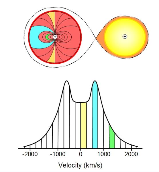
| Above:
Top: a map of a CV as seen from above, in plane view
(inclination = 0); bottom: a double-peaked spectral line, the height of which is the light intensity and the horizontal axis shows velocity of the material emitting the corresponding part of the line. We could plot wavelength instead on the horizontal axis, as the shift in wavelength is proportional to velocity. The shaded regions on the spectral line correspond to the shaded regions of the disc. That is, we have mapped the velocities onto the disc. The higher velocities are seen in the innermost regions of the disc, which equate to the wings of the spectral line, when that part of the disc is moving along our line of sight. Negative velocities indicate motion away from the observer, positive velocities towards. Although the inner parts of the disc are hotter and brighter, the outer regions have a much larger surface area and so contribute more to the brightness of the whole image. Thus, the faster moving inner regions emits lower total light intensities and so the intensity drops off at the wings of the line. |
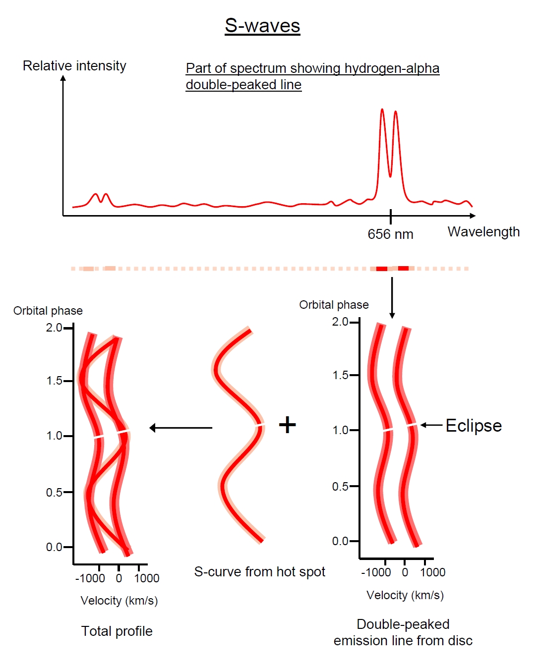
| Above:
the observation of s-waves. Notice the break at phase =
1 where the disc and bright spot are eclipsed by the donor star: the edge of the disc approaching us is eclipsed first. The use of S-waves. Thus, we can obtain an s-wave for every observable feature in the disc, though the bright-spot s-wave is the most obvious. The amplitude of the s-wave gives us the velocity of that component - the faster it moves the larger the height (width in our view) of the wave from peak to trough. For example, this has shown that the speed of the bright-spot is neither equal to the lower speed of the outer disc, nor the higher speed of the mass-transfer stream, but somewhere in-between the two. This shows that as the stream moves from the donor star to the accretion disc, it impacts the disc and slows dramatically, and this sudden conversion of kinetic energy into heat causes the bright-spot to shine so brightly. From these speeds, and given the fact that the material is moving in circular Keplerian orbits, we can obtain two velocity components - the component of velocity along our line-of-sight (y-velocity) and that at right angles to it (x-velocity). This allows us to construct a sort of 2D picture of the disc by plotting y-velocity against x-velocity (what we call velocity-space). This is Doppler tomography and it gives us a tomogram. We can not go the whole way and produce an actual 2D image of the disc in space, since that would mean going from the 1D information in the spectral lines, to a 2D image, and again many uncertainties exist due to the missing information. However, tomograms do assist in visualising discs and may be combined with other methods to build-up a more complete picture. Some example sketches of tomograms are shown below: |
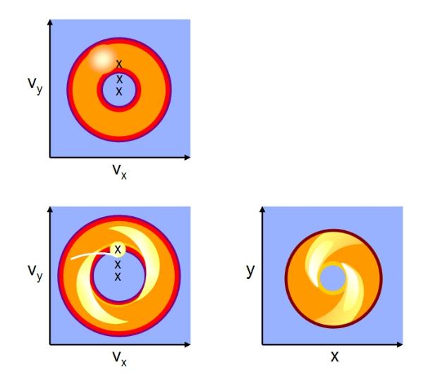
| It
was analysis of the tomogram, obtained by observations
of the spectrum that lead to the discovery that the accretion disc of IP Pegasi contains a spiral-shock pattern. This is caused by perturbation of the disc by the donor star's gravity and this pattern rotates more-or-less in-sync with the binary. This shock pattern corresponds to uneven temperatures of the disc. We make no assumptions as to the effect on the disc shape (such as warping the disc or causing it to bulge). (Note that although this pattern adds a certain patchiness to the disc, it is no more patchy than it needs to be to fit the data). To better visualise the relationship between velocity coordinates on a tomogram and space coordinates on the actual disc, consider the diagram below: |
Top
left: a tomogram of a CV showing the
velocity components of the disc and hot spot.
The topmost X marks the centre of the donor
(secondary) star; the middle X marks the centre
of mass of the system (about which the
components revolve); the bottom-most X marks
the centre of the white dwarf. The system and
disc in a tomogram is inside-out (the inner disc
rotates faster than the outer). Bottom left:
another tomogram showing a spiral shock
pattern. The accretion stream is also indicated.
Bottom right: the model of the spirally
shocked-disc viewed in normal spatial
coordinates, this model will produce the
tomogram on the bottom left.
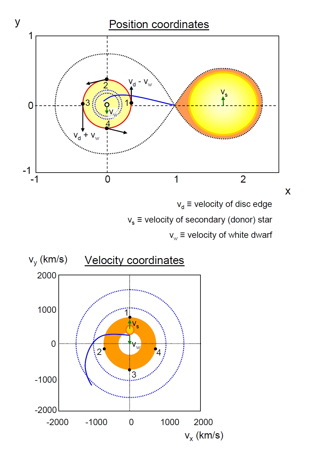
| In
the above diagram, note how positions 1 to 4 on the disc
map to the tomogram. The velocity of point 1 is equal to the velocity of the disc at this point minus the velocity of the white dwarf which is swinging towards us. This velocity is entirely in the positive y-direction, and so the x- component of the velocity on the tomogram is zero. Point 2 has negative x-velocity due entirely to relative motion of the disc, but it also has a small negative y-velocity due to motion of the white dwarf. See if you agree with the velocities of points 3 and 4 as represented on the tomogram. Note that the tomogram turns the disc inside-out, as indicated by the blue dotted circles, and also note the position of the accretion stream (solid blue arc). The centre of the tomogram has zero velocity in both directions (0,0) and corresponds to the centre of mass of the system, around which everything revolves. This assumes that the binary as a whole is not moving towards or away from the observer (or that the effects of such motion have been subtracted). Note also, that although we can go from spatial coordinates to the velocity-coordinates of the tomogram, it is NOT so easy to go in reverse: from a tomogram to the spatial coordinates, since there are many possible spatial arrangements that produce the same tomogram. That is why the research literature goes through the trouble of plotting tomograms instead of spatial coordinates! However, combining Doppler tomography with eclipse mapping may provide additional clues, although some assumptions may need to be made in reconstructing the actual disc geometry. Disc Anomalies We have already seen a disc with a spiral-shock pattern. Other anomalies suggested by observations and/or theoretical calculations include warped discs, thick discs (toruses), optically thin (translucent) and optically thick (opaque) discs, unstable discs and tilted discs. For example, dwarf novas undergo periodic outbursts, each lasting about 3 days, due to disc-instability causing the disc to suddenly heat-up and brighten. Some also show periodic superoutbursts, especially bright outbursts that each last about 14 days. One possible explanation for this is the disc temporarily becomes elliptical. The light-curve of these possibly elliptical discs reveals a superhump, much larger than the usual orbital hump due to the bright spot, in addition to eclipses. These superhumps appear during a superoutburst and then gradually fade away over a number of orbits, presumably as the disc returns to its stable circular state. Some systems, however, exhibit permanent superhumps, and one possible explanation is that these have tilted discs which slowly precess like a spinning top. Also departing from the standard circular thin-disc model are binary systems with magnetar accretors - that is in which accretion takes place onto a white dwarf or neutron star with a very powerful magnetic field. If the field is very strong then no disc will form and the accretion stream will simply split and travel directly to the two poles of the white dwarf where it will emit brightly as it forms columns of in-falling plasma on the star's poles which emit supersonic shock-waves. These systems are called polars. If the magnetic field is not quite so strong, then it disrupts the disc near to the white dwarf, forming veils that sweep-down as curtains onto each pole, but further out a disc may still form, so that the disc is overall incomplete. These systems are called intermediate-polars. We shall explore these systems in a future article. We may also explore the nature of disc instabilities in more detail in a future update. Disc Instability and Outbursts: thermal-viscous instabilities A dwarf nova outbursts is a sudden brightening of a cataclysmic variable by about 100-fold. These bright episodes or outbursts are more-or-less periodic, occurring every 100 days or so, they are only approximately periodic, sometimes an outburst occurs up to about 20 days early or late. The average period varies from binary to binary. Studies of eclipsing binaries (eclipse mapping) have shown that it is the disc that brightens, not the secondary (donor) star and not the bright spot. The fact that the bright spot remains at more-or-less constant brightness during an outburst shows that mass transfer rates are also approximately constant and so the disc does not brighten simply because more mass transfer takes place. Models have been developed to explain these instabilities of accretion discs. These models incorporate instabilities in viscosity and temperature. Viscosity of accretion discs is partly due to the random diffusion of molecules in the disc, which transfers momentum within the disc as the molecules mix. This is normal fluid viscosity, however models suggest that this type of viscosity alone is insufficient. The apparent high viscosity of accretion discs is much higher and this anomalous viscosity is called alpha-viscosity. One explanation of this is magneto- hydrodynamic turbulence (magnetic turbulence). The material in accretion discs is, at least some of the time, significantly ionised, that is many of the atoms (mostly hydrogen) lose their electrons and the material becomes a plasma. Since the ionised particles are electrically charged they move along magnetic field lines (spiralling around them - see particle paths) and rarely move across magnetic field lines. Similarly, moving charged ions generate a magnetic field. The result is that the plasma becomes coupled to the magnetic field, dragging the field with it, and conversely being dragged along by the field. (This depends also how fast the plasma is flowing, if it is moving fast enough then it will drag the field around with it, but if moving too slowly then it will be dragged along by the field). Material in the inner disc is orbiting faster than material further out, in the outer disc. Imagine a magnetic field line joining two packets of plasma, one further toward the disc centre than the other. The packet, pocket or blob of plasma further in will move faster than the outer packet and the field line becomes stretched and pulls on the slower moving outer packet, transferring angular momentum from the inner packet to the outer packet. This causes the outer packet to move further out, whilst the inner packet which has lost momentum spirals further in. Eventually the magnetic field lines stretch to breaking point and the lines rupture and reconnect in a different configuration, leaving the two packets now disconnected. This is the essential angular momentum transfer system that allows most of the material to lose angular momentum, spiral in and become accreted on the white dwarf's surface, whilst a smaller amount of matter spins off into outer space, carrying away the excess angular momentum which would otherwise stop material moving in to the white dwarf. This phenomenon is called magnetic breaking. The accretion disc is never completely uniform. The mass accretion rate varies slightly and the density of the disc may vary, causing local pockets of increased density where material begins to pile up. With more matter radiating energy (as it loses gravitational potential energy) these pockets of higher density are hotter. The increase in temperature increases the ransom diffusion of the atoms or ions, and thus increases the viscosity (by increasing momentum transfer). This increased viscosity increases the loss of angular momentum and the material in the pocket falls inwards faster, reducing the density and thus lowering the temperature and maintaining the balance. In this way a disc can remain stable, apart from small local fluctuations. However, if the temperature in the pocket rises to about 7000 K or above, the hydrogen atoms begin to ionise (becoming a plasma). Photons (particles or quanta of light) interact more with the electrically charged ions than they do with the neutral atoms, absorbing and scattering the light which then finds it difficult to escape - the region becomes opaque (optically thick). In the range of temperatures over which ionisation occurs, any further release of energy goes mostly into ionising the gas, rather than heating the material, and the opacity increases very strongly with small increases in temperature (opacity is proportional to the temperature to the power of 10). Since more radiation gets trapped inside the pocket, this raises the temperature slightly, causing a further dramatic increase in opacity, leading to a further temperature increase, and so on, in a runaway heating effect. Although the increase in temperature tends to accelerate inward movement of the material, as before, tending to drain the pocket and reduce its temperature, this effect is outweighed by the opacity effect on temperature and the pocket gets hotter, causing a local thermal instability. This also heats neighbouring regions of disc material and a wave of heating spreads across the entire disc in a domino effect - the thermal instability now affects the whole disc, spreading out from the local region of instability that initiated it. If, when the disc was in its stable or quiescent state, the mass transfer rate, from the donor star to the disc, was low enough, then material would have had time to fall inwards and tends to accumulate in the inner disc. In this case the local instability starts in the inner disc and spreads outwards in an inside-out heating wave. If, however, the mass transfer rate was too high, then material piles up in the outer disc, before it has time to fall inwards by losing angular momentum, In this case the thermal instability begins in the outer disc and spread inwards in an outside-in heating wave. In both cases the wave pushes material inwards until the inner disc becomes the densest. When the disc is hot enough such that its atoms are more-or-less totally ionised (ending the unstable runaway phase of slight increases in temperature causing large increases in opacity and hence temperature) it settles down into a new equilibrium in which the rate of accretion is higher than when the disc was quiescent. The disc is hot and much brighter than before, it is in a state of outburst. The elevated accretion rate exceeds the mass transfer rate and the disc begins to empty as material is dumped on the white dwarf. This emptying reduces the density of the disc, lowering its temperature and the disc returns to a state of quiescence, during which it slowly replenishes.
The gravitational potential energy well is steeper closer to the white dwarf, so material in the inner disc radiates more heat for every meter it moves inwards towards the white dwarf than material further out. This means that the minimum density of material required to cause instability is lower in the inner disc. This means that as the disc drains the density passes below critical first in the outer disc and so a cooling-wave begins in the outer disc and moves inwards. Eventually material will accumulate and the disc will enter another phase of instability and enter another outburst. This is why cataclysmic variables are so-named: their brightness varies dramatically! (though semi-predictably). The disc is flip-flopping between these two stable states, hot an cool, as a result of transient instabilities (heating and cooling waves). At least, this is the theory, and it certainly explains the variable nature of the discs. Suggested Reading
|
Article updated: 24 Nov 2018